Market equilibrium
Demand shows us the quantity demanded by consumers at various
prices.
Supply shows us the quantity supplied by the firms
at various prices.
However, demand by itself, or supply by itself cannot
tell us what the price will be in the market.
We can, however, answer this question by using demand
and supply together.
Market equilibrium (contd.)
The price that will eventually be realized in a market
is one at which quantity demanded equals quantity
supplied.
This price, \( p_{e} \) where quantity demanded equals quantity
supplied, is called the equilibrium price; and the
corresponding quantity is called the equilibrium
quantity.
The reason \( p_{e} \) is called the equilibrium price
is that when price equals \( p_{e} \), as long as there
is no change in the underlying conditions that affect
demand and supply, there is no upward or downward pressure
on price.
For any price other than \( p_{e} \) there is an upward
or downward pressure on price depending on whether price
is below \( p_{e} \) or above \( p_{e} \).
Market equilibrium: Graphical representation
Equilibrium price = $4.50
Equilibrium quantity = 300
Why is $6.00 not an equilibrium price?
Presence of surplus (quantity supplied > quantity demanded)
will cause a downward pressure on prices.
Sellers will reduce prices to sell more.
Why is $3.00 not an equilibrium price?
Presence of a shortage (quantity supplied < quantity demanded)
will cause an upward pressure on prices. Buyers will
offer more money and sellers will increase prices.
Solving for equilibrium price and quantity
(Chapter 4, Problem 1 of Acemoglu et al.)
What is the equilibrium price?
Example: Solve for equilibrium price and
quantity.
Suppose demand is given by:
$$
Q_{d} = 1000 - 200 P
$$
and, supply is given by:
$$
Q_{s} = 800 P
$$
where, \( Q \) is the quantity of oranges in a day and
\( P \) is the price per orange (measured in dollars).
Solve for the market equilibrium.
Applications of Market Equilibrium
Using the market equilibrium framework to understand
the effect of various events on prices and quantities.
Example 1: (Chapter 4, Problem 6 of Acemoglu et al.)
There is a sharp freeze in Florida that damages the orange
harvest.
1. How will this affect the price and quantity of oranges?
2. How will this affect the price and quantity of orange juice?
Example 2: (Chapter 4, Problem 5 of Acemoglu et al.)
Brazil is the world's largest coffee producer.
(See
the article on worldatlas.com)
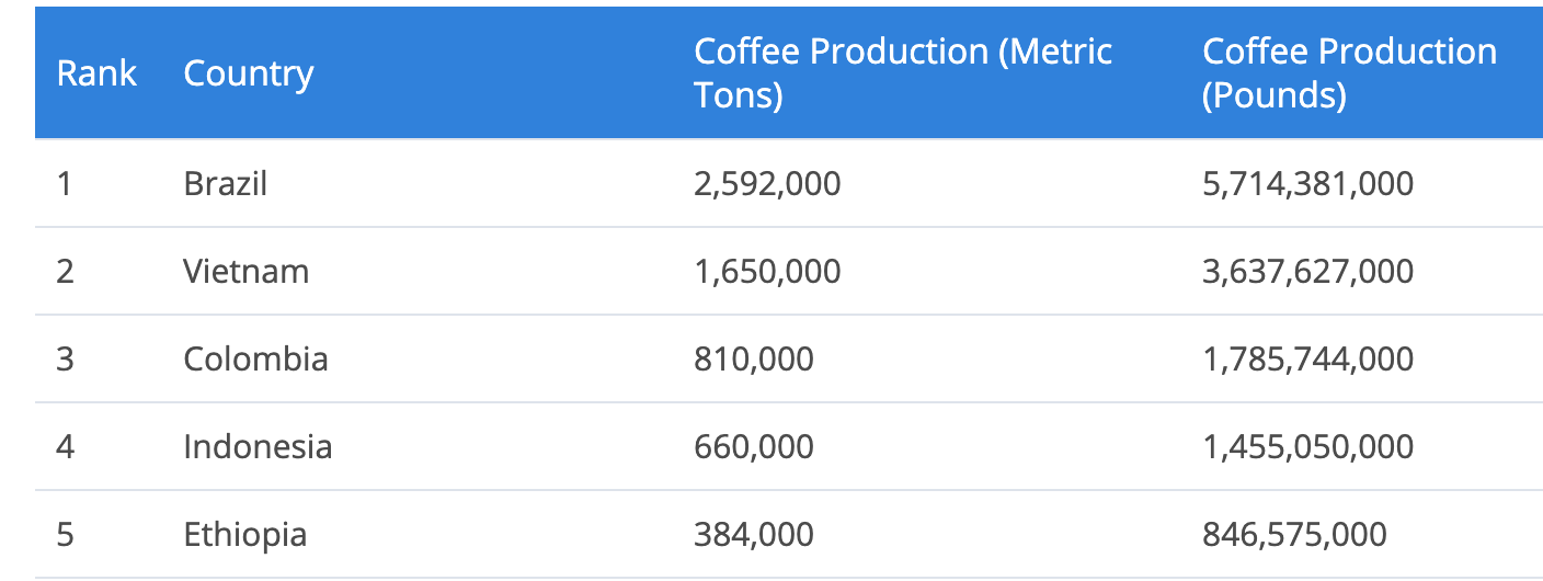
A severe drought in 2013-14 damaged Brazil's coffee crop. The price of
coffee beans doubled in the first three months of 2014.
How do you think this affected the equilibrium price and quantity of tea?
Example 3: (Chapter 4, Problem 8 of Acemoglu et al.)
Land in Sonoma, California can be used either to grow grapes for
Pinot Noir wine or to grow Gravenstein applies. If there is a permanent
rightward shift in demand for Pinor Noir, how will this affect
the equilibrium price and quantity of Gravenstein apples?
Example 4: (Chapter 4, Problem 3 of Acemoglu et al.)
Suppose that a pest attack on the tomato crop increases
the cost of producing ketchup. In addition, a mild winter
causes cattle herds to be unusually large, causing the
price of hamburgers to fall.
What will be the effect on equilibrium price and quantity
of ketchup? Assume that hamburgers and ketchup are
complements.
Effect of per-unit taxes and Tax Incidence
Suppose a per-unit tax is to be imposed in a market. It can be
imposed on the buyers, or on the sellers. How will the
two parties be affected in each case?
Are the buyers better off when the tax is imposed on the
sellers instead of the buyers?
Are the sellers better off when the tax is imposed on
the buyers instead of the sellers?
By using our model of the market we shall see that
the effect on buyers and sellers does not depend on whom
(sellers or the buyers) the tax is imposed.
Original equilibrium
Equilibrium price = $3.50.
Equilibrium quantity = 350 units
Tax on buyers of $1 per unit
Equilibrium before tax:
price = $3.50, quantity = 350.
Equilibrium after tax:
price = $3.00, quantity = 300.
Amount paid by the consumer:
$3.00 + $1.00 = $4.00.
Amount received by the seller:
$3.00.
Tax on sellers of $1 per unit
Equilibrium before tax:
price = $3.50, quantity = 350.
Equilibrium after tax:
price = $4.00, quantity = 300.
Amount paid by the consumer:
$4.00.
Amount received by the seller:
$4.00 - $1.00 = $3.00
Welfare effects of taxes
Before we can study the welfare effects, we need to know
how we can measure welfare.
A commonly used approach in Economics is to define
Welfare/Social Surplus as:
Consumer surplus (CS)
+ Producer surplus (PS)
+ (Government Revenue - Government Expenditure)
+ (Externality benefits - Externality Costs)
We have not yet discussed the notion of externality, and
you can ignore it for now. We will talk about it after a few
classes.
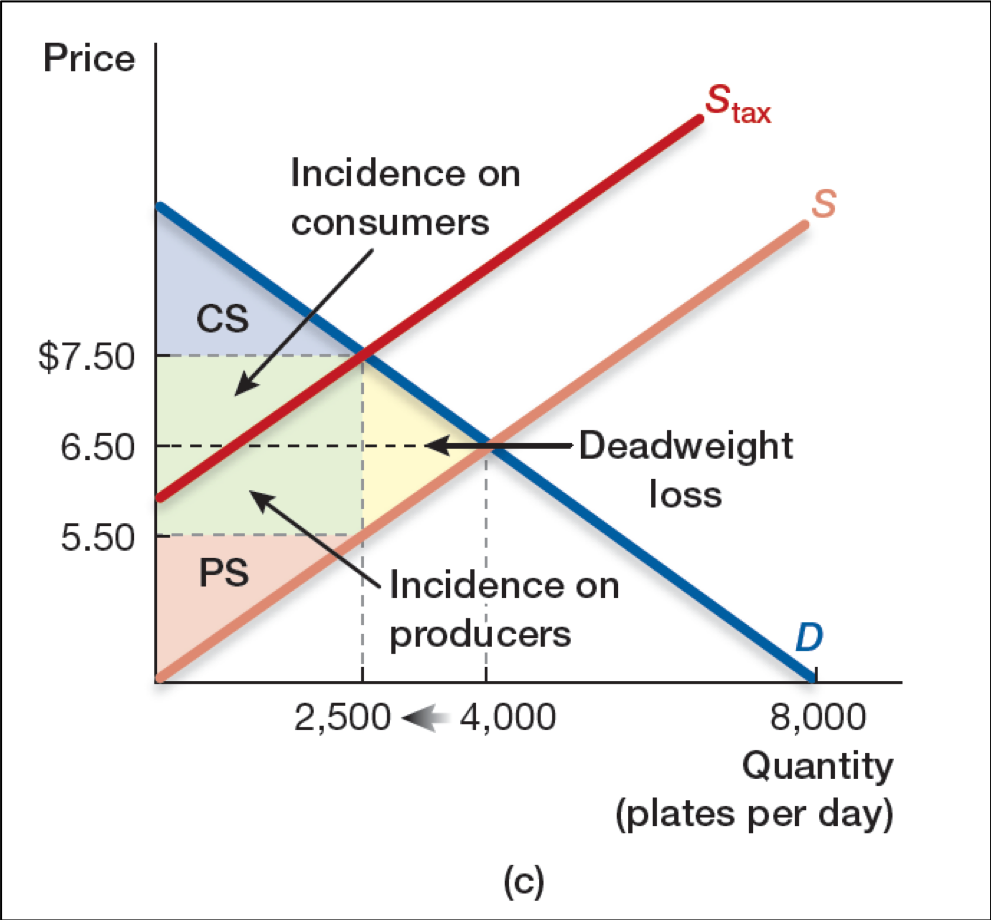
Welfare effects of taxes (continued)
The figure to the left shows the effect of a tax on sellers.
Identify the welfare effects of this tax using the labeled areas.
Consumer surplus before tax:
1 + 2 + 3 + 4
Consumer surplus after tax:
1
Hence, change in consumer surplus:
- 2 - 3 - 4.
Welfare effects of taxes (continued)
Producer surplus before tax:
5 + 6 + 7
Producer surplus after tax:
2 + 5
Hence, change in producer surplus:
2 - 6 - 7
Welfare effects of taxes (continued)
Government Revenue before tax
None.
Government Revenue after tax:
3 + 6
Hence, Change in Goverment Revenue
3 + 6
Welfare effects of taxes (continued)
Putting changes in consumer surplus, producer surplus, and
government revenue together, we obtain
Change in Welfare
= - 2 - 3 - 4 + 2 - 6 - 7 + 3 + 6
= - 4 - 7
Welfare effects of taxes (continued)
The
yellow highlighted
area (4 + 7) is the welfare loss due to taxes.
This loss is referred to as the
deadweight loss due to taxes.
Calculate the numerical values of changes in CS, PS
Tax Revenue and Welfare
Further practice
For practice with change in equilibrium outcome read chapter 4
and problems at the end of Chapter 4.
For the welfare effect of taxes find the changes in CS, PS, Tax Revenue
and Welfare in the following figure.
Demand and Supply responsiveness and Tax incidence
We know that how the tax burden is shared between buyers and sellers
does not depend on whether the tax is imposed on sellers or on buyers.
But, how is the burden shared? Is it shared equally?
Is most of it borne by the sellers, or by buyers?
What determines how the burden is shared?
How the tax burden is shared between buyers and sellers
depends on how responsive the quantity demanded and supplied are
to prices.
For example, consider necessities: products that people consume
because they need them, as opposed to because they provide
pleasure/entertainment. Bypass surgery is one example.
Next few slides illustrate how the burden shared depends on
demand responsiveness given the responsiveness of supply.
Demand responsiveness and the sharing of tax burden
(Demand 1)
The figure to the left shows the supply before tax (\(S_{0}\))
and the supply after tax (\( S_{1} \)).
What is the tax per unit? How
much of it is paid by the consumer, and how much is paid by the seller?
Tax per unit = $20.
Eqm. price before tax = $60.
Eqm. price after tax = $70.
Consumer's share of the burden per unit = $70 - $60 = $10.
Seller's share of the burden per unit = $20 - $10 = $10.
Consumer's share 50% of the tax burden.
Demand responsiveness and the sharing of tax burden
(Demand 2)
The figure to the left shows the supply before tax (\(S_{0}\))
and the supply after tax (\( S_{1} \)).
What is the tax per unit? How
much of it is paid by the consumer, and how much is paid by the seller?
Tax per unit = $20.
Eqm. price before tax = $60.
Eqm. price after tax = $75.
Consumer's share of the burden per unit = $75 - $60 = $15.
Seller's share of the burden per unit = $20 - $15 = $5.
Consumer's share 75% of the tax burden.
Demand responsiveness and the sharing of tax burden
(Demands 1 and 2)
Summary: Demand 2 is less responsive than Demand 1. Hence,
sellers pass on relatively greater burden of the tax
(75% instead of 50%) on consumers.
Effect of a price ceiling (A)
What is the welfare consequence of a price ceiling
at \(p_{ceilA}\)?
There is a welfare loss denoted by area
\(ABE\).
Effect of a price ceiling (B)
What is the welfare consequence of a price ceiling
at \(p_{ceilB}\)?
A price ceiling above the equilibrium price
has no welfare consequence. Market price will be
the same regardless of whether or not there is a ceiling.
Effect of a price floor (B)
What is the welfare consequence of a price floor
at \(p_{floorB}\)?
There is a welfare loss denoted by area
\(ABE\).
Effect of a price floor (A)
What is the welfare consequence of a price floor
at \(p_{floorA}\)?
A price floor below the equilibrium price
has no welfare consequence. Market price will be
the same regardless of whether or not there is a
price floor.


